CW Bandwidth described
|
CW Bandwidth described |
|
An Intuitive Explanation of CW Bandwidth by Mark Amos, W8XR How much bandwidth does it take to send Morse code?
When the question of CW* bandwidth is discussed there are often inconsistencies and inaccuracies sprinkled in among the facts. And, while technical explanations can be found, they are typically laced with difficult mathematics. In researching the topic, I found that there was a lack of simple, intuitive explanations. I hope this article serves that need.
Topics that we’ll cover: - Production of radio frequency CW - Morse Code keying - The keying “envelope” - Rise and fall times - Keying speed, baud rates - Carrier bandwidth - CW bandwidth
First, some basic foundation material about radio, Morse code speed, baud rates and keying for those of you who haven’t spent much time in this arena.
What does it take to send Morse code via radio waves? - some kind of a radio frequency oscillator to create a carrier frequency - an amplifier to buffer and amplify the oscillator output - a feed line and antenna to couple the signal from the amplifier to the void - a way to turn that carrier (CW*) on and off to transmit Morse code.
We won’t talk about the first three here. There are plenty of good books and websites that explain them well – the ARRL Handbook is a great place to start.
One obvious way to turn the carrier on and off is to use a key between an oscillator and an antenna. Alternatively, as in some early radios, the key might turn an oscillator on and off as we tap out our message. Or, it might interrupt the signal from the oscillator to the amplifier. It could also turn the amplifier on and off. It could use a combination of these. Regardless of how it’s done, this keying is what imparts information onto an otherwise steady (and information free) carrier.
A key is a switch – it’s either on or off. If you were to tap out a series of dits on a key hooked up to your transmitter and look at the key’s terminals with an oscilloscope you’d see something that looks like a square or rectangular wave. If you’ve been around long enough, you might even have heard one or two radios that had oscillators or amplifiers that were directly keyed.
“Modern” radios modify the shape of this keying waveform so that it doesn’t turn on and off instantaneously. Its transitions are rounded off so that they are less abrupt. We’ll be talking a lot about this shape. It’s often referred to as the “keying envelope.”
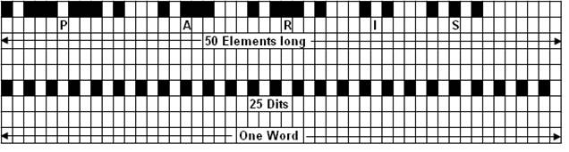
In Morse code there is a “standard word” used in speed measurement. It’s made of the letters, “PARIS.” If it takes you one minute to send PARIS, then you’re sending at one word per minute. The dits, dahs and spaces of PARIS add up to exactly 50 element lengths long (Figure 1.) (The last seven empty elements are an “inter-word” space.)
Fig. 1. “Standard” word PARIS and a simpler test word
Of course there are many possible combinations that would result in a 50 element length word – PARIS is just one that is used as a “standard.”
For the analysis below we will use an alternative and very simple 50 element length word: a string of 25 dits. Add up all the dits and the separating spaces and you get a 50 element length word. You could use any test word – ultimately the results would be similar – but this simple 25 dit string might make the following discussion a little easier to understand.
If we send our test word at the ridiculously high speed of 60 WPM (Words Per Minute) we get one word per second.
If you had a computer before high speed internet access was the norm, you used a modem. Modem speed is measured in terms of “baud rate”. Typical baud rates for modems started out at 110 baud in the 1970s and increased quickly through 300, 1200, 9600, 192000 and 56000 baud in the 90’s. How fast is 60 WPM in terms of baud? This requires a look at the technical definition of “baud.” It’s not critical that you understand baud rate – I’m just providing this information for comparison purposes.
One baud is equal to one bit of information (or one “state change”) per second. There are two state changes per dit in our test word – one where the carrier turns on, the other where it turns off.
While there are people that can copy code faster than this, there aren’t many. The record is just over 75 WPM. Our test word at 60 WPM is about the cross-over point where other digital modes start making more sense than the on/off keying (OOK) of Morse code.
A common conversion factor for WPM to baud is .83. So, 60 WPM * .83 is about 50 baud. 12 WPM is about 10 baud. One of the slowest RTTY baud rates (45.45 bauds) is close to our 60 WPM test keying rate. (In computer signaling, the term bps has replaced baud as a transmission speed measurement. This can get confusing because it is possible to encode more than one bit into a state change. We’ll ignore that complication for this discussion.)
You might be thinking, “Well, if baud is state changes per second, then wouldn’t real Morse code words have different baud rates than this test word at 60 WPM?” Yes, in fact there could be many 50 element length words each with different baud rates because of the different number of transitions. Morse code has variable length letters so the conversion to baud and bits per second is a bit odd. But it doesn’t really matter to this discussion, so we’ll ignore this complication too… I’ve only mentioned it here to give you a frame of reference. If you need to do a WPM to BAUD conversion, just use .83 bauds / WPM and you’ll be close.
When we send our 25 dit “test word” at 60 WPM, we will key and un-key the carrier 25 times per second (“25 Hz”, or “25 cycles per second “.)
One way to think of this is that we’re “amplitude modulating” our carrier with a 25 Hz keying envelope. Just turning the carrier off and on is a very simple type of modulation. It’s also very noisy and inefficient – it requires a lot of bandwidth. We’ll talk about how much bandwidth a little later.
However, as we know, Morse code can be a very bandwidth efficient medium if we’re careful.
Being conscientious amateurs, we would never key our transmitter with a “square” (on/off) keying envelope. That would be seriously “hard” keying – the kind that causes annoying “key clicks”. Instead let’s try a softer kind of keying, rounding off the sharp corners of this square, on/off keying envelope.
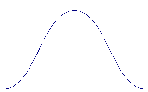
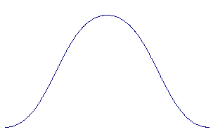
In fact, let’s start with the “softest” possible keying. We’ll use a “raised cosine” shaped wave for our keying envelope. It will gently increase our carrier from 0 to 100% and then back down again.
Technically, the softest possible shape is actually a Gaussian noise curve. As shown in Figure 2., they are really the same shape with different names.
Fig. 2 Raised Cosine Waveform Fig. 3 Gaussian Waveform
So, using the very soft keying envelope from Figure 2 (or Figure 3…), the carrier starts out with zero amplitude, slowly rises, and accelerates as it climbs through 50%. Then its rate of climb decelerates until it gets to 100% carrier amplitude. This rise from 0 to 100% forms a kind of S-shaped curve (a “sinusoidal” curve.) After reaching 100%, it begins to drop off. This drop-off accelerates down through 50% and finally the rate of change slows down as the end of the keying envelope is approached. The changes to the amplitude of the carrier are smoothly changing throughout.
If we do this in 40 milliseconds, we will have sent one “dit” at 60 WPM (we’ll do the calculation for this a little later.)
This would be impossible for a human to copy. If we sent 25 of these (our test word), at 60 WPM the sound would “run together” and the result would be an unintelligible 25 Hz hum. (Under laboratory conditions, using a computer with digital signal processing software, the computer might be able to “read” these 25 dits, but not you or I.)
In any case, copy-able or not, this keying envelope results in the minimum possible bandwidth necessary to key a carrier at 60WPM.
Let’s not confuse this minimum possible bandwidth with bandwidth required for readability. What we’re talking about here is the minimum possible bandwidth that occurs when you key a carrier at 60 WPM with a raised cosine keying envelope. (We’ll talk about bandwidth required for effective receiving some other time.)
So, how much bandwidth does it take? We need some simple mixer theory to talk about this.
As you should remember from studying for your amateur license, when you modulate (or mix) one signal with another, you get the sum and difference of the two signals. Often the two original frequencies tag along and the modulating signal is typically removed by filtering.
So, a 1 MHz carrier modulated by this soft 25 Hz keying waveform, results in 4 resulting frequencies: 1.) 999,975 Hz (the difference: 1 MHz - 25 Hz) 2.) 1,000,025 Hz (the sum: 1 MHz + 25 Hz) 3.) 1,000,000 Hz (the carrier) 4.) 25 Hz (the modulation frequency) – this signal won’t make it out of your amplifier, much less your antenna…
So, the bandwidth this mixed signal uses is: 1,000,025 - 9,999,975 = 50 Hz. The sum and difference signals are what create the “sidebands” of the signal. The sum results in the upper sideband and the difference makes up the lower sideband. The carrier in the middle doesn’t take up any bandwidth (and doesn’t contain any information.)
As I said, using this soft keying envelope, Morse code would be extremely difficult for other people to copy. In order to make it more readable, we need to “harden” the keying.
For now, let’s use rise time and fall time to describe the keying “hardness.” (The “shape” of the rise and fall is important too – but we’ll keep the shape constant for now and continue to use parts of a raised cosine shaped envelope.)
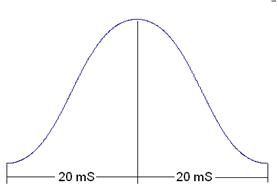
Using the softest of all possible keying envelopes, the Gausian envelope, the rise time for a dit is 20 mS and the fall time is 20 mS. When we send a string of 25 of these dits, this makes up what amounts to a 40 mS wavelength. (We can check our work by taking the reciprocal of the frequency to get the wavelength – that is we divide 1 by 25. This comes out to .040 seconds or 40 mS; half of it is rise time and half of it is fall time (Fig. 4.)
For this kind of soft keying, we’ll call anything above 50% “on” and anything below 50% “off”.
Fig. 4 One “Dit” at 60 WPM (25 Hz keying envelope.)
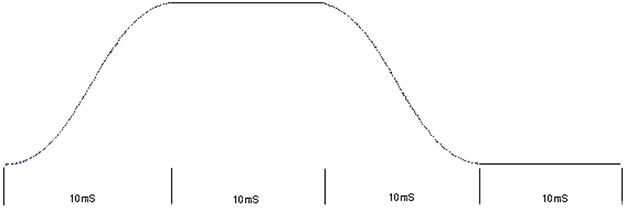
What if we halve the rise time and fall time to 10 mS but leave the frequency the same?
We’ll get (Figure 5.): 10 mS rise time 10 mS where the signal is at 100% 10 mS fall time 10 mS with the signal at 0.
Since the frequency is the same, 25 Hz, this whole envelope has to add up to 40 mS. We’ve just sort of “stretched out” the parts of the envelope where the carrier is 100% and where it’s 0%. But we’ve also narrowed the raised cosine parts for a sharper rise and fall. See figure 5.
Figure 5. 10 mS rise, 10 mS at 100%, 10 mS fall and 10 mS at 0 (Still 25 Hz – 60 WPM)
During the times when the envelope is steady (at 100% and 0) the carrier is not taking up any bandwidth: if we transmit an unchanging 1MHz carrier it won’t take up any bandwidth. This is difficult for a lot of people to accept. It seems counterintuitive (“There must be SOMETHING there taking up bandwidth”), but it’s true.
Put another way: the only time that the sidebands push out and take up bandwidth is during a change in the amplitude of the carrier. That is, during the time that the envelope is going up or down (where the amplitude of the carrier is increasing or decreasing.) Ideally, when transmitting CW, this only happens during the rise time and fall time of the keying envelope**.
Even this smooth raised cosine envelope changes the amplitude of the carrier, albeit slowly and gracefully – no jagged edges here. This changing envelope causes the sidebands to push out either side of the carrier.
OK, now let’s dig just a little deeper.
The width of the sidebands (the bandwidth) has to do with the “steepness” of the keying envelope; how fast it is changing the carrier’s amplitude. By increasing the slop of our keying waveform, we’re increasing the required bandwidth. Signaling theory folks would argue that it’s the rate of modulation – the 25 Hz modulating signal in our example – that causes the sidebands. I’ve heard a number of arguments about this assertion.
You’re welcome to look at it this way, but consider this: what is really changing when the modulation rate changes? It’s the steepness of the rise time and fall time of the keying envelope. Here’s an example.
What if we double our initial keying rate from 60 WPM to120 WPM (that is, increase our modulating frequency from 25 Hz to 50 Hz)? What would the leading and trailing edges look like?
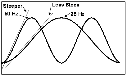
This is easier to see than it is to talk about. Take a look at a 25 Hz cosine shaped wave overlaying a 50 Hz cosine shaped wave in Figure 6.
Fig. 6 It’s the “Steepness” that counts.
Notice anything interesting about how steep the 50 Hz wave is as it goes from 0 to peak?
You might say the rate of change is “twice as steep” as in the 25 Hz wave – and you’d be right. In order to fit 50 cycles into the same second that our 25 Hz signal fits in, each 50 Hz wave has to have “steeper” sides than the 25 Hz waves – in fact, twice as steep. Again, it’s the rate of change of the carrier due to the keying envelope that counts. The slope, or the rate of change, is a measure of the “steepness” of the rise or fall time. For a modulating (or keying) waveform, twice as steep means twice the bandwidth.
Some might still argue that the increase in the modulation rate is causing this.
Of course there’s a kernel of truth there. If you increase the rate of modulation, you increase the steepness of the modulating wave form (as is evident in Figure 6.) But, it’s actually the steepness of the rising and falling envelope that causes the sidebands (and consequent bandwidth) not the signaling rate. If you had only one wave at this frequency, the bandwidth required would be exactly the same as the continuous train of waves in our example.
Technically, it’s not just the steepness of the rise time and fall time. More precisely, it’s the rate of change of any part of the envelope. For instance, if instead of a nice smooth rise from 0 there’s an abrupt change, this abrupt change will increase the bandwidth. A saw-tooth, triangular or stepwise envelope would cause a much higher bandwidth signal than our raised cosine envelope. If the carrier is modulated in some other way the bandwidth could also increase (for instance if the signal has some “chirp”) but in this analysis we’re only considering bandwidth due to the keying envelope.
You need to get to the point where you can say, with conviction: “It’s the shape of the keying envelope that causes a keyed CW signal to take up bandwidth. An un-keyed/un-modulated CW signal takes up no bandwidth.”
How can we determine how wide our signal will be based on the rise and fall times of the keying envelope? This section talks about a way to estimate this.
When we harden the keying by increasing the slope of the rising or falling part of the keying envelope, we’re pushing out the sidebands as if we were modulating our carrier with a wave that has the same slope and shape as the rising and falling parts of the modulation envelope. This is a little tricky, but an example should help.
In the first scenario above, we halved the rise and fall time to 10 mS apiece but kept the keying rate the same. By cutting the rise and fall time in half, it’s as if we’re now modulating our carrier with a 50 Hz sine wave (even though the rise time and fall time are separated by periods of no change.) The sidebands push out to +- 50 Hz, requiring 100 Hz of total bandwidth to send this same 60 WPM word.
Another way to say this: if we keep the rise time and fall time of our envelope and take out any parts where the envelope is not changing (when it’s at 100% and 0% for instance), we can figure out this waveform’s frequency (based on its wavelength) and use that to estimate required bandwidth. So, for instance, a 50 Hz sine wave has a rise time and fall time of 10 mS each (1 / 50 is 20 mS.) If our envelope has the same rise time and fall time as a 50 Hz sine wave, and it’s rise and fall have the same shape as the rise and fall of a 50 Hz sine wave, then we can treat it like a 50 Hz signal to compute bandwidth.
Remember: when the keying envelope isn’t changing, there are no sidebands and no bandwidth – sidebands and bandwidth only occur during the times when the keying envelope is changing.
If we halve the rise and fall times again (to 5 mS), it’s as if we’re modulating our carrier with a 100 Hz waveform (5 mS rise time + 5 mS fall time = 10 mS; 1/10 mS = 100 Hz). The sidebands go out to +- 100 Hz for a total of 200 Hz bandwidth.
Of course in the real world, not many radios use smooth Gaussian keying, as we do here. Typically they use a resistor-capacitor “filter” used to soften up the rise and fall. Why is this still done? The engineering isn’t that hard anymore - it’s a matter of economics: it would cost more per radio for manufacturers to add a Gaussian keying envelope.
An RC filter has sharper edges and consequently causes more bandwidth to be used. It’s obviously better than just using a square keying envelope. However it’s still pretty wide and if the rise time and fall times are less than 5mS or so, it will be pretty “clicky” even on some high-end radios.
Ok, so how much bandwidth would a “square” keying wave take?
Way too much. The rise and fall times of a square wave are “infinitely” steep. This kind of keying results in a very wide signal with lots of noise with every key down and key up.
It’s as if you’re modulating your carrier with a very high frequency signal – sidebands are pushed out to infinite bandwidth. Well, maybe not infinite, but a lot more than the other amateurs up and down the band deserve. If you’re doing this on 40 meters, some of your key clicks could be making it up to the 20 meter band -- or maybe even your phone or your neighbor’s TV, depending on how much power you’re trying to pump out.
Not only is this inefficient – there is wasted power in those “infinite” sidebands – in most parts of the civilized world it’s illegal. The exact bandwidth is tricky to calculate, because of things like the bandwidth of your transmitter, filters that might be in the signal path, your amplifier linearity, the width of the pass-band of your tuner, the bandwidth of your antenna, etc.
Regardless, it’s wide enough to get you in trouble. So pay attention to your keying envelope. Don’t key that homebrew rig with a square envelope or any envelope that has a rise time or fall time less than 5 mS or so. Also, if possible the rise and fall should be shaped like our raised cosine curve. If they’re exponential curves (like you get with an RC filter) you will be taking up more bandwidth than is absolutely necessary.
Here are a couple of key takeaways:
- If you take nothing else from this article, you should be able to say with confidence “The bandwidth of a typical CW signal depends on the shape of the keying envelope.” - The hardness of the keying is greatly influenced by the rise and fall time of the keying envelope. A rise and fall time of 5mS or more will result in a readable signal at reasonable bandwidth. - Sidebands of a CW signal are caused by keying (an unmodulated carrier requires no bandwidth.) - You can estimate the bandwidth required by analyzing the shape of the keying envelope (“removing” the parts that are unchanging and calculating the frequency of the remaining portions.) This applies with “soft” keying. Using “harder” keying increases the required bandwidth dramatically. - Lots of people like to argue about these points even if they don’t really understand them. It’s best to just “walk away” from these arguments, unless you just like to argue. Little exchange of knowledge is likely to occur, even if it is somewhat entertaining…
*Technically, CW means “Continuous Wave.” When radio amateurs talk about CW they’re really talking about on/off keying (OOK) of a continuous wave. Certainly there’s nothing “continuous” about a keyed carrier; it stops and starts all the time. As mentioned above technically, CW doesn’t take ANY bandwidth at all if it’s not being modulated. In this article, we use the term CW in the amateur sense.
**Of course in the real world there are complications, like phase noise, jitter, FM, etc. but that’s another story and doesn’t really add to this discussion in any meaningful way.
|